Mapping centromeres using Optical Map data

Optical mapping has become rather common for applications ranging from genome assembly improvement and validation to structural variation discovery. Validation of the rice genome using Optical map data also helped map centromeres and even span one centromere. However, in some cases centromeres have been found to correspond to regions that have poor mapping of optical maps, presumably due to the presence of tandem repeats that lack unique restriction sites. Without the availability of genetic linkage maps or other evidence, those working with NGS based draft assemblies have speculated that large gaps in the optical map correspond to centromeres or other repeats.

The Human genome has a higher quality as well as availability of various other resources such as genetic linkage maps, BAC's, FISH etc in addition to the availability of optical mapping data. Centromeres have been mapped in the human genome with various other methods and provides an ideal case to investigate the patterns(or lack thereof) shown by optical maps near centromeres. Optical map data for the human and mouse genome from published studies have been made available as bigBed files. This provides a unique resource to understand the behavior of optical maps near centromeres.

First we download the bigBed files for the human genome Hg38 and convert it to bed12 format. This can then be converted to bed format using the convert perl script

 wget ftp://ngs.sanger.ac.uk/production/grit/track_hub/hg38/om_align_GM10860.bigBed  
 wget ftp://ngs.sanger.ac.uk/production/grit/track_hub/hg38/om_align_GM15510.bigBed  
 wget ftp://ngs.sanger.ac.uk/production/grit/track_hub/hg38/om_align_GM18994.bigBed  
 for i in om_align_GM10860 om_align_GM15510 om_align_GM18994  
 do  
 bigBedToBed "$i".bigBed "$i".bed  
 perl convertBed.pl "$i".bed > "$i"_full.bed  
 done  

Perl script called covertBed.pl to convert bed12 to bed format.

 #!/usr/bin/perl  
 my $bed12file = $ARGV[0];  
 open(FILE1, $bed12file);  
      while($header1=<FILE1>) {  
      chomp $header1;  
      my @parts=split(/\t/,$header1);  
      my @parts2=split(/\,/,$parts[10]);  
      my @parts3=split(/\,/,$parts[11]);  
      my $arrSize = @parts2;  
           for($i=0;$i<$arrSize;$i++){  
           $start=$parts[1]+$parts3[$i];  
           $end=$start+$parts2[$i];  
           print "$parts[0]\t$start\t$end\t$parts2[$i]\n";  
           }  
      }  
 close FILE1;  

We next create 50Kb windows across the human genome to analyze the distribution of cut sites in the Optical map.

 mysql --user=genome --host=genome-mysql.cse.ucsc.edu -B -A -D hg38 -e 'select chrom,size from chromInfo' > chromhg38.genome  
 bedtools makewindows -g chromhg38.genome -w 50000|sort -k1,1 -k2,2n > 50kb.wins  

All 3 Optical maps are combined and the mean of the fragment lengths as well their counts are tabulated in 50Kb windows.

 cat *_full.bed|sort -k1,1 -k2,2n > full_all.bed  
 bedtools map -a 50kb.wins -b full_all.bed -c 4 -o mean -null NA > all.mean  
 bedtools map -a 50kb.wins -b full_all.bed -c 4 -o count -null NA > all.count  

Analysis of these numbers across each chromosome suggests that mean fragment size might be a better predictor of centromeres than the count. The position of the centromeres is obtained from the UCSC tables using below command:

 mysql --user=genome --host=genome-mysql.cse.ucsc.edu -B -A -D hg38 -e 'select chrom,chromStart,chromEnd from centromeres'|grep -v "chromStart" > centromeres.hg38.genome  

Running below R code will create graphical images showing the position of the centromeres by red lines and the mean fragment size by blue dots.

 for (chr in c("chr1","chr2","chr3","chr4","chr5","chr6","chr7","chr8","chr9","chr10","chr11","chr12","chr13","chr14","chr15","chr16","chr17","chr18","chr19","chr20","chr22","chrX"))  
 {  
 read.table(file="all.mean",header=F)->M  
 read.table(file="centromeres.hg38.genome",header=F)->C  
 interleave <- function(v1,v2)  
 {  
 ord1 <- 2*(1:length(v1))-1  
 ord2 <- 2*(1:length(v2))  
 c(v1,v2)[order(c(ord1,ord2))]  
 }  
 jpeg(paste(chr,"_OM.jpeg",sep=""))  
 plot(M$V2[M$V1==chr],M$V4[M$V1==chr],xlab="Position along chromosome",ylab="Mean fragment length in Optical Map",main=chr,col="blue",pch=16)  
 lines(interleave(C$V2[C$V1==chr],C$V3[C$V1==chr]),rep(0.2,length(interleave(C$V2[C$V1==chr],C$V3[C$V1==chr]))),col="red",lwd=5)  
 dev.off()  
 }  

Based on below figures, it can be hypothesized that on chr1, chr2, chr3(to certain extent), chr7, chr9, chr11(to certain extent),chr12,chr13, chr14,chr15 and chr20 the mean optical fragment size goes up near centromeres.

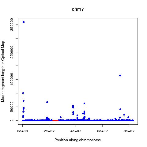
Based on the above analysis can one conclude that it is possible to map Centromeres using Optical mapping data? Far from it, the many false positives and lack of signal in many cases are worrying. The following questions are of importance:

 

1. How does the quality of the genome assembly in the regions adjoining the centromere affect the ability to map centromeres?
2. How does the enzyme used and repeat content and base composition of the centromere affect the precision of attempts aimed at mapping the centromere?